Before starting with this, I wanted to ensure that if at any point you feel that you’re not able to understand or grasp what is written on this page, that is totally understandable. These concepts are better understood when practised, not theoretically. So, if you’re not able to understand something, don’t worry, we’ll be coding using these in the next few days, and you’ll get a hang of it.
This guide has been written keeping in mind that you have a basic understanding of C++ and have written some code in it. If you haven’t, I would recommend you to start with that first. Although the language used is C++, the concepts are the same in any language, so you can follow along with any language you’re comfortable with. The syntax might change, but the concepts remain the same.
Data Structures and Algorithms are the building blocks of any program. They help you write efficient code and solve complex problems. Most essential for systems programming, they are also used in other core software engineering roles.
Time Complexity
Time complexity is a measure of the amount of time an algorithm takes to run as a function of the length of the input. It is used to analyze the efficiency of an algorithm. The time complexity of an algorithm is usually expressed using Big O notation. Big O notation describes the upper bound of the time complexity of an algorithm. It is used to describe the worst-case scenario of an algorithm. Other notations include Big Omega and Big Theta, which describe the lower bound and average case of an algorithm, respectively.
- O(1) - Constant time complexity
- O(log n) - Logarithmic time complexity
- O(n) - Linear time complexity
- O(n log n) - Linearithmic time complexity
- O(n^2) - Quadratic time complexity
- O(n^3) - Cubic time complexity
Algorithms with lesser time complexity are more efficient than those with higher time complexity. For example, an algorithm with O(1) time complexity is more efficient than an algorithm with O(n) time complexity. We would want our tasks to be completed quickly, like in a sec, rather than waiting for n seconds.
Data Structures
Data structures are a way of organizing and storing data so that it can be accessed and modified efficiently. They are used to store and manipulate data in a computer program.
Primitive Data Structures
Primitive data structures allow you to store a single data value. These include:
- Integers
- Floats
- Characters
- Booleans
- Pointers
Non-Primitive Data Structures
Non-primitive data structures allow you to store multiple data types. There are two types of non-primitive data structures:
- Linear Data Structures
- Non-Linear Data Structures
Linear Data Structures
As the name suggests, the linear data structures can store data in a linear dimension. There are two types of linear data structures:
- Static
- Dynamic
Elements are stored sequentially. These include:
- Arrays - Static
- Vectors - Dynamic
- Linked Lists - Dynamic
- Stacks - Dynamic
- Queues - Dynamic
Non-Linear Data Structures
Elements are stored in a non-sequential manner. These include:
- Trees
- Graphs
- Hash Tables
- Heaps
- Tries
etc.
Data Structures in C++
-
Arrays - Arrays are a collection of elements of the same data type. They are static in nature, meaning that the size of the array is fixed; you can’t change it once declared. The elements are stored in contiguous memory locations. The index of the first element is 0.
int arr[5] = {1, 2, 3, 4, 5};
cout<<"The first element is:"<<arr[0]<<endl;
[1, 2, 3, 4, 5] -
Vectors - Vectors are similar to arrays, but they are dynamic. You can change the size of the vector once declared. They are implemented using arrays. They are part of the Standard Template Library (STL) in C++.
#include <vector>
vector<int> v = {1, 2, 3, 4, 5};
cout<<"The last element is:"<<v[v.size()-1]<<endl;

v.push_back(6);
The benefit of using vectors is that you don’t have to worry about the size of the vector, you can keep adding elements to it. Usually, the size is always doubled when the vector is full.
-
Linked Lists - Linked lists are a collection of elements called nodes. Each node contains data and a pointer to the next node. They are dynamic. There are three types of linked lists:
-
Singly Linked List - Each node contains data and a pointer to the next node. The last node points to NULL. It can be traversed only in one direction.
Here is an example of a singly linked list:
struct Node { int data; Node* next; }; int main() { //Creating a linked list Node* head = new Node(); head->data = 1; head->next = NULL; //Adding elements to the linked list for(int i = 2; i<=5; i++) { Node* temp = new Node(); temp->data = i; temp->next = NULL; Node* temp1 = head; while(temp1->next!=NULL) { temp1 = temp1->next; } temp1->next = temp; } } -
Doubly Linked List - Each node contains data, a pointer to the next node, and a pointer to the previous node. It can be traversed in both directions.
struct Node { int data; Node* next; Node* prev; }; -
Circular Linked List - The last node points to the first node. It can be traversed in both directions.
struct Node {
	int data;
	Node* next;
};
int main(){
	//Creating a circular linked list
	Node* head = new Node();
	head->data = 1;
	head->next = head;
	//Adding elements to the circular linked list
	for(int i = 2; i<=5; i++) {
		Node* temp = new Node();
		temp->data = i;
		temp->next = head;
		Node* temp1 = head;
		while(temp1->next!=head) {
			temp1 = temp1->next;
		}
		temp1->next = temp;
	}
}
 A Singly Linked List with data value as integers
Linked Lists allow you to insert and delete elements in O(1) time complexity, whereas arrays or vectors take O(n) time complexity. The disadvantage of linked lists is that you can’t access elements randomly, you have to traverse the list to access an element.
Arrays/ Vectors: O(1) to access an element, O(n) to insert/delete an element Linked Lists: O(n) to access an element, O(1) to insert/delete an element
In almost all cases, vectors are preferred over arrays and linked lists because of their dynamic nature and the ability to access elements randomly.
-
-
Stacks - Stacks are a collection of elements that follow the Last In First Out (LIFO) principle. They have two main operations: push and pop. The push operation adds an element to the top of the stack, and the pop operation removes the top element from the stack. (A stack of PS5 CDs, a stack of papers, etc.)
#include <stack>
stack<int> s;
s.push(1);
s.push(2);
s.push(3);
cout<<"The top element is:"<<s.top()<<endl;
s.pop();
cout<<"The top element is:"<<s.top()<<endl;
Simple representation of a stack runtime with push and pop operations.
You can also use vectors/ arrays/ linked lists to implement stacks manually. Try implementing a stack using vectors.
Stacks are used in applications where the order of elements is important, such as in compilers, browsers, etc. In compilers, the stack is used to store the operators and operands of an expression, and the order in which they are popped determines the order of evaluation. Refer to this link for more information. A function call is also implemented using a stack. When a function is called, the address of the next instruction is pushed onto the stack, and when the function returns, the address is popped from the stack. All of this becomes clear when you start coding.
The std::stack in C++ is implemented using a deque (double-ended queue). A deque is a type of queue where elements can be added or removed from both the front and the rear. It is implemented using arrays. The std::stack is a wrapper around the std::deque.
Stacks - O(1) to access the top element, O(1) to insert an element, O(1) to delete an element
-
Queues - Queues are a collection of elements that follow the First In First Out (FIFO) principle. They have two main operations: enqueue and dequeue. The enqueue operation adds an element to the rear of the queue, and the dequeue operation removes the front element from the queue. (A queue of people waiting at Comicon, a book signing by JKR, a queue of cars at a toll booth, etc.)
#include <queue> queue<int> q; q.push(1); q.push(2); q.push(3); cout<<"The front element is:"<<q.front()<<endl; q.pop(); cout<<"The front element is:"<<q.front()<<endl;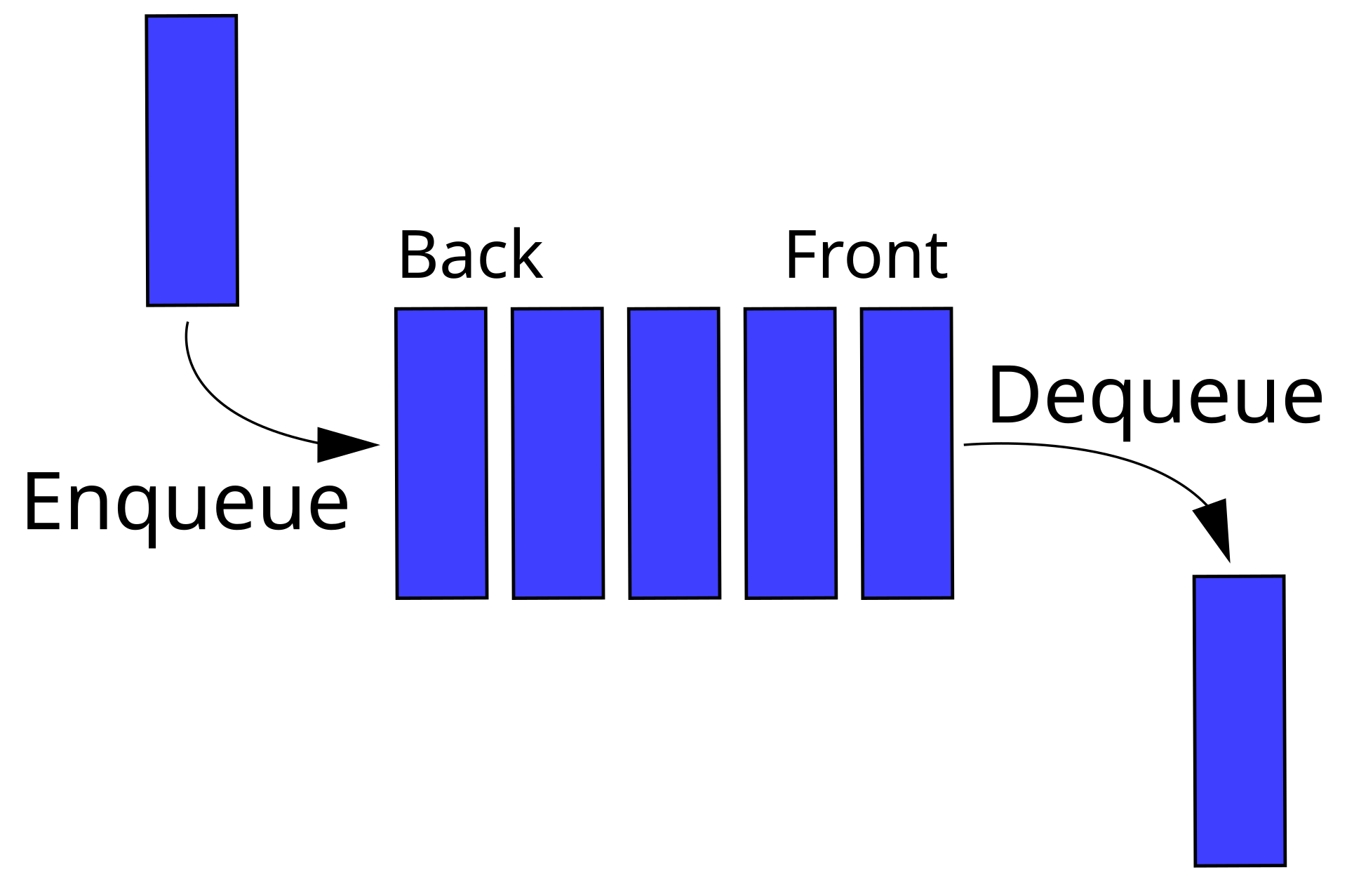 Representation of a FIFO (first in, first out) queue
Try implementing a queue using vectors/ arrays/ linked lists.
Queues are also used when the order of elements is important, such as in printers, operating systems, etc. In printers, the queue is used to store the print jobs, and the order in which they are dequeued determines the order of printing. In operating systems, the queue is used to store the processes, and the order in which they are dequeued determines the order of execution.
The std::queue in C++ is implemented using a deque (double-ended queue). A deque is a type of queue where elements can be added or removed from both the front and the rear. It is implemented using arrays. The std::queue is a wrapper around the std::deque.
Queues - O(1) to access the front element, O(1) to insert an element, O(n) to delete an element
-
Priority Queues - Priority queues are a type of queue where each element has a priority associated with it. The element with the highest priority is dequeued first. They are implemented using heaps. Heaps are a type of binary tree where the parent node is greater than the child nodes. They are used in Dijkstra’s algorithm, Prim’s algorithm, etc.
#include <queue> priority_queue<int> pq; pq.push(1); pq.push(2); pq.push(3); cout<<"The top element is:"<<pq.top()<<endl; pq.pop(); cout<<"The top element is:"<<pq.top()<<endl; -
Deques - Deques(Double-ended queues) are a type of queue where elements can be added or removed from both the front and the rear. They are used in applications where elements need to be added or removed from both ends, such as in a sliding window, etc.
#include <deque> deque<int> dq; dq.push_front(1); dq.push_back(2); dq.push_front(3); cout<<"The front element is:"<<dq.front()<<endl; cout<<"The rear element is:"<<dq.back()<<endl; -
Circular Queues - Circular queues are a type of queue where the rear of the queue is connected to the front of the queue. They are used in applications where the queue needs to be circular, such as in a round-robin scheduling algorithm, etc.
#include <queue>
queue<int> q;
q.push(1);
q.push(2);
q.push(3);
cout<<"The front element is:"<<q.front()<<endl;
q.pop();
cout<<"The front element is:"<<q.front()<<endl;
-
-
Hash Tables - Hash tables are a type of data structure that stores key-value pairs. They are implemented using hash functions. The key is hashed to generate a unique index, and the value is stored at that index. They are used in applications where fast access to elements is required, such as in databases, compilers, etc.
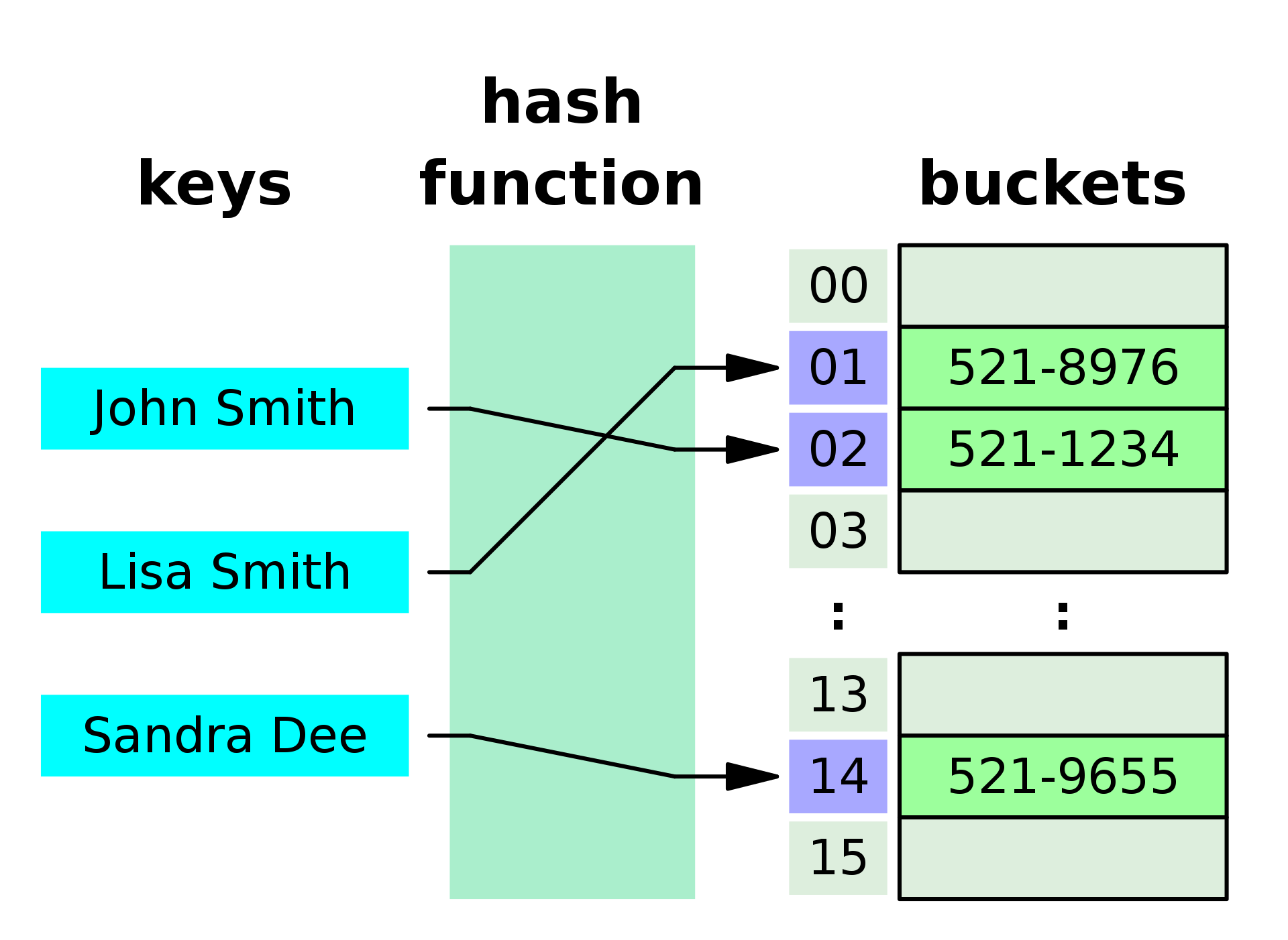 A small phone book as a hash table
-
Unordered Map - There is no order maintained in the keys. The keys are hashed to generate a unique index, and the value is stored at that index. The keys are unique.
#include <unordered_map>
unordered_map<int, string> um;
um[1] = "one";
um[2] = "two";
um[3] = "three";
cout<<"The value of key 2 is:"<<um[2]<<endl;
Hash Tables - O(1) to access an element, O(1) to insert an element, O(1) to delete an element
-
Ordered Map - The keys are ordered based on the key values.
#include <map>
map<int, string> m;
m[1] = "one";
m[2] = "two";
m[3] = "three";
cout<<"The value of key 2 is:"<<m[2]<<endl;
Ordered Maps - O(log n) to access an element, O(log n) to insert an element, O(log n) to delete an element
-
Unordered/ Ordered Set: A set is a collection of unique elements. Same as the other, but with unique elements.
-
-
Tree - A tree is a collection of nodes(vertices) connected by edges. The nodes are arranged in a hierarchical order.
 This unsorted tree has non-unique values (e.g., the value 2 existing in different nodes, not in a single node only) and is non-binary (only up to two children nodes per parent node in a binary tree). The root node at the top (with the value 2 here), has no parent as it is the highest in the tree hierarchy.
-
Binary Tree - A tree where each node has at most two children.
struct Node { int data; Node* left; Node* right; }; -
Binary Search Tree - A type of binary tree where the left child is smaller than the parent node, and the right child is greater than the parent node. The binary search tree is used to search for elements in O(log n) time complexity. The binary search tree can be traversed in three ways:
-
AVL Tree - A type of binary search tree where the difference in height between the left and right subtrees of each node is at most one. The AVL tree is used to maintain the balance of the tree. The AVL tree is used in applications where the height of the tree needs to be minimized, such as in databases, etc.
-
Red-Black Tree - A type of binary search tree where each node is colored red or black. The red-black tree is used to maintain the balance of the tree. The red-black tree is used in applications where the height of the tree needs to be minimized, such as in databases, etc.
-
B-Tree - A type of tree where each node can have more than two children. The B-tree is used to maintain the balance of the tree. The B-tree is used in applications where the height of the tree needs to be minimized, such as in databases, etc.
-
Trie (Prefix Tree) - A trie is a type of tree where each node represents a character. The trie is used to store strings. The trie is used in applications where the search for strings is important, such as in dictionaries, etc.
-
Segment Tree - A segment tree is a type of tree where each node represents a range of elements. The segment tree is used to perform range queries on an array. The segment tree is used in applications where range queries are important, such as in databases, etc.
-
Fenwick Tree - A Fenwick tree is a type of tree where each node represents a range of elements. The Fenwick tree is used to perform range queries on an array. The Fenwick tree is used in applications where range queries are important, such as in databases, etc.
Segment tree -
- query in O(logN)
- preprocessing in O(N)
- Pros: less time complexity.
- Cons: More amount of code compared to the other data structures.
Fenwick tree -
- query in O(logN)
- preprocessing in O(NlogN)
- Pros: the shortest code, less time complexity
- Cons: Fenwick tree can only be used for queries with L=1, so it is not applicable to many problems.
-
Suffix Tree - A suffix tree is a type of tree where each node represents a suffix of a string. The suffix tree is used to store strings. The suffix tree is used in applications where the search for strings is important, such as in dictionaries, etc.
-
Binary Indexed Tree - A binary indexed tree is a type of tree where each node represents a range of elements. The binary indexed tree is used to perform range queries on an array. The binary indexed tree is used in applications where range queries are important, such as in databases, etc.
-
Huffman Tree - A Huffman tree is a type of tree where each node represents a character and its frequency. The Huffman tree is used to compress data. The Huffman tree is used in applications where data compression is important, such as in file compression, etc.
-
Quad Tree - A quadtree is a type of tree where each node represents a quadrant of a 2D space. It tree is used to partition a 2D space. The quadtree is used in applications where the partitioning of a 2D space is important, such as in image processing, etc.
-
Octree - An octree is a type of tree where each node represents an octant of a 3D space. The octree is used to partition a 3D space. The octree is used in applications where the partitioning of a 3D space is important, such as in 3D graphics, etc.
-
Heap - A heap is a type of tree where each node is greater than or equal to its children. The heap is used to maintain the maximum or minimum element at the root node. The heap is used in applications where the maximum or minimum element needs to be maintained, such as in priority queues, etc.
Trees are used in applications where the hierarchical relationship between elements is important, such as in file systems, family trees, etc.
Trees - O(log n) to search for an element, O(log n) to insert an element, O(log n) to delete an element
-
-
Graph - A graph is a collection of nodes(vertices) and edges. The edges connect the nodes. There are two types of graphs:
 A directed graph with three vertices (blue circles) and three edges (black arrows).
- Directed Graph - The edges have a direction associated with them. The direction is from one node to another. Tree is a type of directed graph.
- Undirected Graph - The edges do not have a direction associated with them. The direction is bidirectional.
There are two ways to represent a graph:
-
Adjacency Matrix - An adjacency matrix is a 2D array where the rows represent the source nodes and the columns represent the destination nodes. The value at the intersection of the row and column represents the weight of the edge between the source and destination nodes.
int adj[5][5] = { {0, 1, 0, 1, 0}, {1, 0, 1, 0, 0}, {0, 1, 0, 1, 1}, {1, 0, 1, 0, 0}, {0, 0, 1, 0, 0} }; -
Adjacency List - An adjacency list is a collection of linked lists where each node has a list of its adjacent nodes. The linked list can be implemented using vectors or linked lists.
#include <vector>
vector<int> adj[5];
adj[0].push_back(1);
adj[0].push_back(3);
adj[1].push_back(0);
adj[1].push_back(2);
adj[2].push_back(1);
adj[2].push_back(3);
adj[2].push_back(4);
adj[3].push_back(0);
adj[3].push_back(2);
adj[4].push_back(2);
Graphs are used in applications where the relationship between elements is important, such as in social networks, maps, etc. Graphs - O(n) to search for an element, O(1) to insert an element, O(1) to delete an element
-
Suffix Array - A type of array where each element represents a suffix of a string. The suffix array is used to store strings. The suffix array is used in applications where the search for strings is important, such as in dictionaries, etc.
-
Bloom Filter - A bloom filter is a type of data structure that tests whether an element is a member of a set. The bloom filter is used to test the membership of an element in a set. The bloom filter is used in applications where the membership of an element needs to be tested, such as in spell checkers, etc.
-
Skip List - A data structure that allows for fast search, insertion, and deletion of elements. The skip list is used to store elements. The skip list is used in applications where fast search, insertion, and deletion of elements are important, such as in databases, etc.
Algorithms
Algorithms are a set of instructions that are used to solve a problem. There are a million algorithms out there, but the most common ones are:
- Searching Algorithms
- Sorting Algorithms
- Graph Algorithms
- Tree Algorithms
- Dynamic Programming
- Greedy Algorithms:
- String Algorithms:
Searching Algorithms
Linear Search
Linear search employs a straight-forward search technique. It keeps on searching the element until found. It is not suitable for large datasets as it has a time complexity of O(n).
int linearSearch(int arr[], int n, int key) {
	for(int i = 0; i<n; i++) {
		if(arr[i] == key) {
			return i;
		}
	}
	return -1;
}
Binary Search
Binary search is a search algorithm that finds the position of a target value within a sorted array. It compares the target value to the middle element of the array. If they are not equal, the half in which the target cannot lie is eliminated, and the search continues on the remaining half until it is successful. It has a time complexity of O(log n).
Ex. [1, 2, 3, 4, 5, 6, 7, 8, 9, 10]
Element to search: 2
- Compare 2 with the middle element 6. 2<6.
- Eliminate the right half. The array becomes: [1, 2, 3, 4, 5]
- Compare 2 with the middle element 3. 2<3. The array becomes: [1, 2]
- Compare 2 with the middle element 2. 2=2. Element found at index 1. (Indexing starts from 0)
int binarySearch(int arr[], int n, int key) {
	int low = 0, high = n-1;
	while(low<=high) {
		int mid = low + (high-low)/2;
		if(arr[mid] == key) {
			return mid;
		}
		else if(arr[mid]<key) {
			low = mid+1;
		}
		else {
			high = mid-1;
		}
	}
	return -1;
}
The only caveat with this is that the array needs to be sorted, else the algorithm won’t work.
Using either of two depends on the size of the dataset and the order. For small datasets, linear search is preferred, and for large datasets, binary search is preferred. If the dataset is sorted, binary search is preferred. If the dataset is unsorted, linear search is preferred.
Sorting Algorithms
Bubble Sort
Bubble sort is a simple sorting algorithm that repeatedly steps through the list, compares adjacent elements, and swaps them if they are in the wrong order. The pass through the list is repeated until the list is sorted. It has a time complexity of O(n^2).
Ex. [5, 3, 8, 6, 2]
- Compare 5 and 3. 5>3. Swap them. [3, 5, 8, 6, 2]
- Compare 5 and 8. 5<8. No swap. [3, 5, 8, 6, 2]
- Compare 8 and 6. 8>6. Swap them. [3, 5, 6, 8, 2]
- Compare 8 and 2. 8>2. Swap them. [3, 5, 6, 2, 8]
- Compare 3 and 5. 3<5. No swap. [3, 5, 6, 2, 8]
- Compare 5 and 6. 5<6. No swap. [3, 5, 6, 2, 8]
- Compare 6 and 2. 6>2. Swap them. [3, 5, 2, 6, 8]
- Compare 6 and 8. 6<8. No swap. [3, 5, 2, 6, 8]
- Compare 3 and 5. 3<5. No swap. [3, 5, 2, 6, 8]
- Compare 5 and 2. 5>2. Swap them. [3, 2, 5, 6, 8]
- Compare 5 and 6. 5<6. No swap. [3, 2, 5, 6, 8]
- Compare 6 and 8. 6<8. No swap. [3, 2, 5, 6, 8]
- Compare 3 and 2. 3>2. Swap them. [2, 3, 5, 6, 8]
- Compare 3 and 5. 3<5. No swap. [2, 3, 5, 6, 8]
- Compare 5 and 6. 5<6. No swap. [2, 3, 5, 6, 8]
- Compare 6 and 8. 6<8. No swap. [2, 3, 5, 6, 8]
Now the array is sorted. The number of passes is n-1, where n is the number of elements in the array.
void bubbleSort(int arr[], int n) {
	for(int i = 0; i<n-1; i++) {
		for(int j = 0; j<n-i-1; j++) {
			if(arr[j]>arr[j+1]) {
				swap(arr[j], arr[j+1]);
			}
		}
	}
}
Selection Sort
It is the simplest sorting algorithm. It works by selecting the smallest (or largest, depending on sorting order) element from the unsorted portion of the array and swapping it with the first unsorted element. It has a time complexity of O(n^2).
Ex. [5, 3, 8, 6, 2]
- Select 2 as the minimum element. Swap it with 5. [2, 3, 8, 6, 5]
- Select 3 as the minimum element. Swap it with 3. [2, 3, 8, 6, 5]
- Select 5 as the minimum element. Swap it with 8. [2, 3, 5, 6, 8]
- Select 6 as the minimum element. Swap it with 6. [2, 3, 5, 6, 8]
void selectionSort(int arr[], int n) {
	for(int i = 0; i<n-1; i++) {
		int minIndex = i;
		for(int j = i+1; j<n; j++) {
			if(arr[j]<arr[minIndex]) {
				minIndex = j;
			}
		}
		swap(arr[i], arr[minIndex]);
	}
}
Insertion Sort
Insertion sort works by building a sorted array from the unsorted portion of the array; it iterates over the array and removes one element per iteration, finds the place the element belongs in the sorted list, and inserts it there. Insertion sort is how you arrange a deck of cards. It has a time complexity of O(n^2).
Ex. [5, 3, 8, 6, 2]
- Select 3. Insert it at the correct position. [3, 5, 8, 6, 2]
- Select 8. Insert it at the correct position. [3, 5, 8, 6, 2]
- Select 6. Insert it at the correct position. [3, 5, 6, 8, 2]
- Select 2. Insert it at the correct position. [2, 3, 5, 6, 8]
void insertionSort(int arr[], int n) {
	for(int i = 1; i<n; i++) {
		int key = arr[i];
		int j = i-1;
		while(j>=0 && arr[j]>key) {
			arr[j+1] = arr[j];
			j--;
		}
		arr[j+1] = key;
	}
}
Merge Sort
This is a divide-and-conquer algorithm. It divides the input array into two halves, calls itself for the two halves, and then merges the two sorted halves. It has a time complexity of O(n log n).
Ex. [5, 3, 8, 6, 2]
- Divide the array into two halves. [5, 3, 8] [6, 2]
- Divide the first half into two halves. [5] [3, 8]
- Divide the second half into two halves.[6] [2]
- Merge the two halves. [3, 5, 8] [2, 6]
- Merge the two halves. [2, 3, 5, 6, 8]
void merge(int arr[], int l, int m, int r) {
	int n1 = m-l+1;
	int n2 = r-m;
	int L[n1], R[n2];
	for(int i = 0; i<n1; i++) {
		L[i] = arr[l+i];
	}
	for(int i = 0; i<n2; i++) {
		R[i] = arr[m+1+i];
	}
	int i = 0, j = 0, k = l;
	while(i<n1 && j<n2) {
		if(L[i]<=R[j]) {
			arr[k] = L[i];
			i++;
		}
		else {
			arr[k] = R[j];
			j++;
		}
		k++;
	}
	while(i<n1) {
		arr[k] = L[i];
		i++;
		k++;
	}
	while(j<n2) {
		arr[k] = R[j];
		j++;
		k++;
	}
}
Quick Sort
Quick sort is a divide-and-conquer algorithm. It picks an element as a pivot and partitions the given array around the picked pivot. There are many different versions of quickSort that pick pivot in different ways. It has a time complexity of O(n^2) in the worst case, but O(n log n) in the average case.
Ex. [5, 3, 8, 6, 2]
- Select 5 as the pivot. [3, 2, 5, 8, 6]
- Select 3 as the pivot. [2, 3, 5, 8, 6]
- Select 8 as the pivot. [2, 3, 5, 6, 8]
int partition(int arr[], int low, int high) {
	int pivot = arr[high];
	int i = low-1;
	for(int j = low; j<high; j++) {
		if(arr[j]<pivot) {
			i++;
			swap(arr[i], arr[j]);
		}
	}
	swap(arr[i+1], arr[high]);
	return i+1;
}
References
- Searching Algorithms
- Binary Search
- Time Complexity: O(log n)
- Space Complexity: O(1)
- Suitable for: Large datasets, sorted arrays.
- Linear Search
- Time Complexity: O(n)
- Space Complexity: O(1)
- Suitable for: Small datasets, unsorted arrays.
- Binary Search
- Sorting Algorithms
- Bubble Sort
- Time Complexity: O(n^2)
- Space Complexity: O(1)
- Suitable for: Small datasets.
- Selection Sort
- Time Complexity: O(n^2)
- Space Complexity: O(1)
- Suitable for: Small datasets.
- Insertion Sort
- Time Complexity: O(n^2)
- Space Complexity: O(1)
- Suitable for: Small datasets.
- Merge Sort
- Time Complexity: O(n log n)
- Space Complexity: O(n)
- Suitable for: Large datasets.
- Quick Sort
- Time Complexity: O(n^2) (worst case), O(n log n) (average case)
- Space Complexity: O(log n)
- Suitable for: Large datasets.
- Bubble Sort
- Graph Algorithms
- Breadth-First Search (BFS)
- Time Complexity: O(V+E)
- Space Complexity: O(V)
- Suitable for: Shortest path, connected components, etc.
- Depth-First Search (DFS)
- Time Complexity: O(V+E)
- Space Complexity: O(V)
- Suitable for: Topological sorting, connected components, etc.
- Breadth-First Search (BFS)
- Tree Algorithms
- Tree Traversal (Inorder, Preorder, Postorder)
- Time Complexity: O(n)
- Space Complexity: O(n)
- Suitable for: Traversing a tree.
- Binary Search Tree (BST) operations (Insertion, Deletion, Searching)
- Time Complexity: O(log n)
- Space Complexity: O(1)
- Suitable for: Searching, sorting, etc.
- Tree Traversal (Inorder, Preorder, Postorder)
- Dynamic Programming
- Longest Common Subsequence (LCS)
- Time Complexity: O(mn)
- Space Complexity: O(mn)
- Suitable for: DNA sequence matching, etc.
- Longest Increasing Subsequence (LIS)
- Time Complexity: O(n^2)
- Space Complexity: O(n)
- Suitable for: Longest increasing subsequence, etc.
- Matrix Chain Multiplication
- Time Complexity: O(n^3)
- Space Complexity: O(n^2)
- Suitable for: Matrix chain multiplication, etc.
- Edit Distance
- Time Complexity: O(mn)
- Space Complexity: O(mn)
- Suitable for: DNA sequence matching, etc.
- Coin Change Problem
- Time Complexity: O(nm)
- Space Complexity: O(n)
- Suitable for: Coin change, etc.
- Fibonacci Series
- Time Complexity: O(n)
- Space Complexity: O(n)
- Suitable for: Fibonacci series, etc.
- Knapsack Problem (0/1 Knapsack)
- Time Complexity: O(nW)
- Space Complexity: O(nW)
- Suitable for: Knapsack problem, etc.
- Longest Common Subsequence (LCS)
- Greedy Algorithms:
- Activity Selection
- Time Complexity: O(n log n)
- Space Complexity: O(n)
- Suitable for: Activity selection, etc.
- Fractional Knapsack
- Time Complexity: O(n log n)
- Space Complexity: O(n)
- Suitable for: Fractional knapsack, etc.
- Dijkstra’s Algorithm (for shortest path)
- Time Complexity: O(V^2)
- Space Complexity: O(V)
- Suitable for: Shortest path, etc.
- Prim’s Algorithm (for minimum spanning tree)
- Time Complexity: O(V^2)
- Space Complexity: O(V)
- Suitable for: Minimum spanning tree, etc.
- Kruskal’s Algorithm (for minimum spanning tree)
- Time Complexity: O(E log V)
- Space Complexity: O(V)
- Suitable for: Minimum spanning tree, etc.
- Huffman Coding
- Time Complexity: O(n log n)
- Space Complexity: O(n)
- Suitable for: Data compression, etc.
- Activity Selection
- String Algorithms:
- String Matching (Naive Algorithm)
- Time Complexity: O(mn)
- Space Complexity: O(1)
- Suitable for: String matching, etc.
- KMP Algorithm
- Time Complexity: O(m+n)
- Space Complexity: O(m)
- Suitable for: String matching, etc.
- Rabin-Karp Algorithm (for substring search)
- Time Complexity: O(mn)
- Space Complexity: O(1)
- Suitable for: Substring search, etc.
- String Matching (Naive Algorithm)
Next?
There is a lot of information in these pages, more than 70% of which you probably won’t need. The important data structures are marked with \b font-weight. The rest are just for your information. Again, it is completely understandable if this becomes too much for you to understand all at once. The best way to understand these is to code them. My primary advice remains the same; try building something cool, and these data structures and algorithms will come to your rescue when stuck. I will keep updating this page, adding more information as we go along.