Ferry - A C compiler for RISC-V
The one who compiles C lang to machine code.
- March 25, 2025

The one who compiles C lang to machine code.
The ferryman is a figure in various mythologies responsible for carrying souls across the river that divides the world of the living from the world of the dead.
JK. This post is the second in a series of posts that explore the world of compilers, interpreters, CPUs and low-level systems. The previous post describes how the CPU works; and how CPUs process and execute instructions. This post explains how the code you write in a high-level language is transformed into machine code that the CPU can understand and execute.
This next section is a quick recap taken from the previous post-Docking Compilers. If you are already familiar with how the CPU works, feel free to skip here.
Compilers and interpreters are tools that convert high-level programming languages into machine code instructions that the CPU can execute. Compilers translate the entire program into machine code before execution, while interpreters translate and execute the program line by line.
For ex.
x = 5;
Can be compiled into assembly code like this:
li x1, 5 // load immediate 5 into register x1
sw x1, 0(x0) // store word 0 at address x0
This assembly code is then translated into machine code, which is a binary representation of the instructions that the CPU can execute. The CPU executes these instructions in a sequence, and the program runs.
While interpreters translate and execute the program line by line. The interpreter:
This allows dynamic typing, interactive debugging, and easier integration with other languages. However, interpreters are generally slower than compilers because they don’t optimize the entire program before execution.
Binary code is run as instructions on the CPU. The CPU executes these instructions in a sequence, and the program runs. Each CPU has its own set of instructions it can execute, known as the instruction set architecture (ISA). The ISA defines the instructions the CPU can execute, the registers it uses, and the memory model it follows. For example, an instruction might look like 00000000000000000000000010000011, which translates to lb x1, 0(x0) in RISC-V assembly. This instruction, specific to the RISC-V ISA, loads a byte from memory into register x1.
Computer architecture is the design of computer systems, including the CPU, memory, and I/O devices. The CPU executes machine code instructions, which are specific to the CPU architecture. CPU architectures like x86, ARM, and RISC-V have different instruction sets and memory models. Each instruction set has its own assembly language and machine code format.
Here’s why it is important to understand computer architecture: Compilers generate machine code specific to the target CPU architecture. The machine code for x86 is different from ARM or RISC-V. Interpreters, on the other hand, are CPU-independent. They translate high-level code into bytecode or an intermediate representation that can be executed on any platform.
Ferry is a simple C compiler written in Rust that compiles to RISC-V assembly. It is not a complete implementation of the C language, but a good starting point for understanding how compilers work.
I would suggest getting a basic understanding of how Rust works, and how to set up a Rust project before diving further. Just the basics. Find the Rust Book here.
Compiling Ferry is a pretty straightforward:
cargo build --release
and use
./target/release/ferry <input_file.c>
to run the compiler.
An assembly file with '<input_file>.s will be generated in the same directory as the input file.
The assembly code can be assembled into machine code using an external assembler like riscv64-unknown-elf-gcc. Or, feel free to use an online assembler like RISC-V Online Assembler.
or
cargo run --release --bin runner -- <input_file.s>
to run the code in Mac OS (Apple Silicon - arm64). This will assemble the code and run it using qemu-riscv64.
Before moving forward, Ferry only supports a subset of C. The following features are supported:
Building a compiler is a complicated task. Ferry takes in a program written in C and generates assembly code for the RISC-V using the following steps:
Source Code --> Parser --> AST --> IR Generator --> IR Optimizer --> Assembly Generator (.s) --> Assembler (.o) --> Linker (executable)
Assume we have a simple C program:
#include <stdio.h>

int main() {
  printf("Hello, World!\n");
  return 0;
}
The following code is the exact implementation of the compiler with abstracted implementations of the steps.
fn compile(file: String) -> Result<bool, String> {
 // Parse the source code
    let mut ast = parse_source(&file)?; // Parse the source code into an AST
 // Perform semantic analysis
    ast = semantic::analyze_semantics(ast)?; // Perform semantic analysis on the AST
 // Generate code from the AST
    ir::generate_ir(&ast)?;
 // Assembly generation
    let assembly = codegen::generate_assembly(&ir)?;
    Ok(true) // Return true to indicate successful compilation
}
The assembly code is platform-dependent, meaning that the same high-level code can be compiled into different assembly codes for different architectures. The assembly code is then assembled into machine code, which is specific to the target CPU architecture. Jump to the Assembly and Linking section to see how the assembly code can be converted into machine code using an external assembler.
The compiler reads the source code and breaks it down into tokens. Tokens are the smallest units of meaning in the code, such as keywords, identifiers, literals, and operators.
pub fn parse_source(source: &str) -> Result<(), String> {
    let tokens = tokenize(source)?;
    let mut _ast = build_ast(&tokens)?;
    Ok(())
}
For our example, the tokens generated from the source code would look like this:
Token Stream:
PreprocessorDirective("#include <stdio.h>") --> header file
Type(Int) --> type of variable
Identifier("main") --> function name
LeftParen --> opening parenthesis
RightParen --> closing parenthesis
LeftBrace --> opening brace
Identifier("printf") --> function name
LeftParen --> opening parenthesis
String("Hello, World!\n") --> string literal
RightParen --> closing parenthesis
Semicolon --> semicolon
Keyword(Return) --> return statement
Number(0.0) --> return value
Semicolon --> semicolon
RightBrace --> closing brace
EOF --> end of file
After tokenization, where the source code is broken into tokens, the syntax analyzer (parser) processes these tokens according to the language grammar rules. As it recognizes valid syntactic structures, it constructs the AST. The AST is the output or result of the syntax analysis process.
Each time the parser recognizes a valid language construct (like an expression, statement, or declaration), it creates the corresponding AST nodes.
The parser uses a recursive descent parsing approach, where each function corresponds to a grammar rule. For example, the parse_expression function handles expressions, while the parse_statement function handles statements. The root level function, parse_program, is responsible for parsing the entire program, which then calls the other parsing functions as needed.
The parse_program function might look like this:
match &self.peek().token_type { // Check the type of the next token
  TokenType::Type(_) => { // If it's a type, parse a declaration
    let declaration = self.parse_declaration()?;
    program.add_child(declaration); // Add the declaration to the program
 }
  TokenType::PreprocessorDirective(_) => { // Else if it's a preprocessor directive, parse it
    let directive = self.parse_preprocessor()?;
    program.add_child(directive); // And the directive to the program
 }
  _ => {
    return Err(format!("Expected declaration, found {:?}.", // Error if neither
    self.peek().token_type));
 }
}
The declaration_parser function would then handle the parsing of variable declarations, function declarations, and other constructs. It would create the appropriate AST nodes for each construct and add them to the program node.
The Abstract Syntax Tree (AST) is a tree representation of the source code. Each node in the tree represents a construct in the source code, such as a variable declaration, function call, or control flow statement. The AST is used to represent the structure of the program and is an intermediate representation that can be further processed by the compiler.
A node in the AST might look like this:
pub struct ASTNode {
    pub node_type: ASTNodeType,
    pub children: Vec<ASTNode>,
    pub value: Option<String>,
}
The parser generates the AST by creating nodes for each construct in the source code. For example, a function call might be represented as a node with the type FunctionCall, and its children would be the arguments passed to the function and the function name.
In our example, the AST for the entire program would look something like this:
AST Structure:
└── Root --> root node
├── PreprocessorDirective: Some("#include <stdio.h>") --> header file
└── FunctionDeclaration: Some("main") --> main function declaration
    ├── Type: Some("Int") --> type of function
    └── BlockStatement: None --> block of code starts
        ├── ExpressionStatement: None --> this node doesn't carry any specific value itself - it's just a container that holds the expression
        │   └── CallExpression: Some("printf") --> function call (from stdio.h)
        │       ├── Variable: Some("printf")  --> function name. During the semantic analysis phase after parsing, the compiler would verify that this identifier actually refers to a callable function.
        │       └── Literal: Some("\"Hello, World!\n\"") --> string literal
        └── ReturnStatement: None --> return statement for the function
            └── Literal: Some("0") --> return value
The semantic analyzer checks the AST for semantic correctness. It verifies that the types of variables and expressions are correct, that functions are called with the correct number and types of arguments, and that variables are declared before they are used. The semantic analyzer also performs type checking and resolves any ambiguities in the code.
It checks for preprocessor directives, variable declarations, function declarations, and function calls, and removes any unnecessary nodes from the AST like the #include directives.
For example, assuming there is a #include<matlab.h> directive in the code, and the code looks like this:
#include <matlab.h>
int main() {
 Matrix m = createMatrix(3, 3); // Function declared in matlab.h
    return 0;
}
The semantic analyzer would check that the createMatrix function is declared in the matlab.h header file and that it is called with the correct number of arguments. It would also check that the Matrix type is defined in the header file and that it is used correctly.
After preprocessing, it might look like:
typedef struct {...} Matrix;
Matrix createMatrix(int rows, int cols);
// ...many more declarations...
int main() {
 Matrix m = createMatrix(3, 3);
    return 0;
}
The linker would then resolve the references to the createMatrix function and the Matrix type, ensuring that they are defined in the correct header file.
In our original example, the semantic analyzer would check that the printf function is declared in the stdio.h header file and that it is called with the correct number of arguments. If any semantic errors are found, the compiler reports them to the user.
In the printf("Hello, World!\n") statement, the semantic analyzer checks that the printf function is called with a string argument. If the argument is not a string, it raises an error.
Two specific functions handle this case:
pub fn check_types(node: &ASTNode, symbol_table: &SymbolTable) -> Result<Type, String> {
  ...
  if value.starts_with('"') {
    Ok(Type::Pointer(Box::new(Type::Char))) // String literal
 } else if value == "true" || value == "false" {
    Ok(Type::Bool)
 } else {
    ...
 }
  ...
}
and
pub fn check_types(node: &ASTNode, symbol_table: &SymbolTable) -> Result<Type, String> {
  ...
  match (target_type, value_type) {
 // Basic types
 (Type::Int, Type::Int) => true,
 (Type::Float, Type::Int) => true, // Implicit conversion
    ...
 // Pointers

 // For box types, recursively check if the inner types are compatible
 (Type::Pointer(target_inner), Type::Pointer(value_inner)) => {
      is_type_compatible(target_inner, value_inner)
 }

 // Functions are compatible if their return types and parameter lists match
    if !is_type_compatible(target_return, value_return) {
      return false;
 }
 }
}
This step raises compile-time errors if the AST is not semantically correct.
The intermediate code generator converts the AST into an intermediate representation (IR). The IR is a low-level, usually platform-independent representation of the code that is easier to optimize and translate into machine code.
AST represents the syntactic structure of the code (closely mirrors source code) while IR represents the semantic operations (closer to what the machine will do). IR is specifically designed for optimizations that are difficult at the AST level. Common optimizations like constant folding, dead code elimination, and loop transformations work better on IR.
IR representations are usually standardized and can be used across different compilers. LLVM IR is a widely used intermediate representation that is used by the LLVM compiler infrastructure. It is a low-level, typed assembly-like language that is designed to be easy to optimize and generate machine code from. It is often represented as a three-address code, where each instruction has at most three operands. An LLVM IR representation of the code might look like this:
@.str = private unnamed_addr constant [14 x i8] c"Hello, World!\00", align 1
define i32 @main() {
entry:
 %call = call i32 (i8*, ...) @printf(i8* getelementptr inbounds ([14 x i8], [14 x i8]* @.str, i32 0, i32 0))
 ret i32 0
}
Compilers typically use multiple IR forms during compilation:
Ferry uses a simple IR representation that is built for the purpose of this compiler. The IR is a tree representation of the code, where each node represents an operation or a value. I could have also used LLVM IR as the intermediate representation, but the learning curve is steep, and I wanted to keep it simple. Doing so would actually have made the compiler more robust and powerful.
The IR would look something like this:
IR Structure:
└── Root --> the root node of the IR
└── Function: Some("main") --> the main function
    └── BasicBlock: None --> the entry block of the function
        ├── Call: Some("printf") --> function call
        │   └── Constant: Some("\"Hello, World!\n\"") --> string literal
        └── Return: None --> return statement
            └── Constant: Some("0") --> return value
Industry Practice:
Modern compilers like LLVM, GCC, and .NET all use sophisticated IR systems:
Rust Language also uses LLVM IR as its intermediate representation. The Rust compiler (rustc) generates LLVM IR from the Rust source code, optimizes it, and then generates machine code for the target architecture.
GCC also uses a similar approach, generating an intermediate representation called GIMPLE, which is then optimized and translated into machine code.
Interpreters like Python and JavaScript engines (like V8) also use intermediate representations. For example, the V8 engine uses an intermediate representation called Ignition bytecode, which is a low-level representation of the JavaScript code that can be executed by the V8 engine.
The generated IR is not always optimal. The optimization phase of the compiler improves the IR to make it more efficient. This can include removing dead code, inlining functions, and optimizing loops. The goal of optimization is to improve the performance of the generated code without changing its semantics.
Ferry uses the following optimizations:
Ferry employs two types of optimizations:
Say our code looks like this:
int main(){
  int i = 0 + 2;
  for (i = 0; i < 10; i++)
  {
    if (i == 5)
      return 0;
  }
}
The optimizer should:
0 + 2 at compile time and replace it with 2.i == 5 to avoid unnecessary iterations.i to 0 in the loop header.i == 5 by adding a return statement.The IR could look like this:
IR Structure (Original):
└── Root
└── Function: Some("main")
    └── BasicBlock: None
        ├── BasicBlock: None
        │   ├── Alloca: Some("i")                           // Allocate space for variable 'i'
        │   └── Store: None                                 // Store initial value to 'i'
        │       ├── BinaryOp: Some("+")                     // Calculate 0+2
        │       │   ├── Constant: Some("0")                 // First operand
        │       │   └── Constant: Some("2")                 // Second operand
        │       └── Variable: Some("i")                     // Target variable
        └── BasicBlock: Some("for")
            ├── Store: None                                 // Loop initialization: i = 0
            │   ├── Constant: Some("0")                     // Value to store
            │   └── Variable: Some("i")                     // Target variable
            ├── BasicBlock: Some("for.header")              // Loop condition check
            │   └── BinaryOp: Some("<")                     // Compare i < 10
            │       ├── Load: None                          // Load value of 'i'
            │       │   └── Variable: Some("i")             // Variable to load
            │       └── Constant: Some("10")                // Upper bound
            └── Branch: None                                // Conditional branch
                ├── BinaryOp: Some("<")                     // Same comparison duplicated
                │   ├── Load: None                          // Load value of 'i' again
                │   │   └── Variable: Some("i")
                │   └── Constant: Some("10")
                └── BasicBlock: Some("for.body")            // Loop body
                    ├── BasicBlock: None                    // If statement block
                    │   └── Branch: None                    // Conditional branch
                    │       ├── BinaryOp: Some("==")        // Compare i == 5
                    │       │   ├── Load: None              // Load value of 'i'
                    │       │   │   └── Variable: Some("i")
                    │       │   └── Constant: Some("5")     // Value to compare against
                    │       └── Return: None                // Early return
                    │           └── Constant: Some("0")     // Return value
                    ├── BasicBlock: None                    // Loop increment block
                    │   ├── Load: None                      // Load value of 'i'
                    │   │   └── Variable: Some("i")
                    │   └── Store: None                     // Store i+1 back to i
                    │       ├── BinaryOp: Some("+")         // Calculate i+1
                    │       │   ├── Load: None              // Load value of 'i' again
                    │       │   │   └── Variable: Some("i")
                    │       │   └── Constant: Some("1")     // Increment by 1
                    │       └── Variable: Some("i")         // Target variable
                    └── Jump: Some("for.header")  // Unconditional jump to loop header
The basic optimizer would then optimize the IR using the following optimizations:
---------Starting Optimization---------
Optimization iteration 1
Folded binary op to constant: 2
Replaced load of i with constant None
Replaced load of i with constant None
Replaced load of i with constant None
Replaced load of i with constant None
Replaced load of i with constant None
CSE: Found duplicate expression: LOAD(VAR(i))
CSE: Found duplicate expression: LOAD(VAR(i))
Optimization iteration 2
Replaced load of i with constant None
Replaced load of i with constant None
Replaced load of i with constant None
CSE: Found duplicate expression: LOAD(VAR(i))
CSE: Found duplicate expression: LOAD(VAR(i))
Optimization iteration 3
Replaced load of i with constant None
Replaced load of i with constant None
Replaced load of i with constant None
CSE: Found duplicate expression: LOAD(VAR(i))
CSE: Found duplicate expression: LOAD(VAR(i))
Optimization iteration 4
Replaced load of i with constant None
Replaced load of i with constant None
Replaced load of i with constant None
CSE: Found duplicate expression: LOAD(VAR(i))
CSE: Found duplicate expression: LOAD(VAR(i))
Optimization iteration 5
Replaced load of i with constant None
Replaced load of i with constant None
Replaced load of i with constant None
CSE: Found duplicate expression: LOAD(VAR(i))
CSE: Found duplicate expression: LOAD(VAR(i))
Optimization complete after 5 iterations
and this is what the optimization would look like:
IR Structure:
└── Root
└── Function: Some("main")
    └── BasicBlock: None
        ├── BasicBlock: None
        │   ├── Alloca: Some("i")                          // Allocate space for variable 'i'
        │   └── Store: None                                // Store initial value to 'i'
        │       ├── Constant: Some("2")                    // OPTIMIZATION: Constant folding of 0+2 to 2
        │       └── Variable: Some("i")                    // Target variable
        └── BasicBlock: Some("for")
            ├── Store: None                                // Loop initialization: i = 0
            │   ├── Constant: Some("0")                    // Value to store
            │   └── Variable: Some("i")                    // Target variable
            ├── BasicBlock: Some("for.header")             // Loop condition check
            └── Branch: None                               // Conditional branch
                ├── BinaryOp: Some("<")                    // OPTIMIZATION: CSE - eliminated duplicate comparison
                │   ├── Load: None                         // OPTIMIZATION: Single load of 'i' (CSE applied)
                │   │   └── Variable: Some("i")
                │   └── Constant: Some("10")
                └── BasicBlock: Some("for.body")
                    ├── BasicBlock: None
                    │   └── Branch: None
                    │       ├── BinaryOp: Some("==")       // Compare i == 5
                    │       │   ├── Load: None             // OPTIMIZATION: Single load of 'i' (CSE applied)
                    │       │   │   └── Variable: Some("i")
                    │       │   └── Constant: Some("5")
                    │       └── Return: None               // Early return
                    │           └── Constant: Some("0")
                    ├── BasicBlock: None
                    │   └── Store: None                    // OPTIMIZATION: Simplified increment
                    │       ├── BinaryOp: Some("+")
                    │       │   ├── Load: None             // OPTIMIZATION: Single load of 'i' (CSE applied)
                    │       │   │   └── Variable: Some("i")
                    │       │   └── Constant: Some("1")
                    │       └── Variable: Some("i")
                    └── Jump: Some("for.header")           // Loop back
While it correctly preserved the program’s structure and performed some basic optimizations like constant folding (0 + 2 → 2), it hasn’t performed the more advanced control flow analysis that would recognize this optimization opportunity. The advanced optimizer would then optimize the IR using the following optimizations:
---------Starting Advanced Optimization---------
Optimization iteration 1
Optimization iteration 2
Optimization complete after 2 iterations

----- Optimization Summary -----
Constants folded: 0
Dead code blocks removed: 2
Common expressions eliminated: 0
Loops optimized: 0
Functions optimized: 0
-------------------------------
and this is what the optimization would look like:
IR Structure (During Advanced Optimization):
└── Root
└── Function: Some("main")
    └── BasicBlock: None
        ├── Alloca: Some("i")                     // Allocate space for variable 'i'
        ├── Store: None                           // OPTIMIZATION: Eliminated dead store (i=2 never used)
        │   ├── Constant: Some("0")               // Store initial loop value directly
        │   └── Variable: Some("i")               // Target variable
        ├── BasicBlock: Some("loop_check")        // OPTIMIZATION: Simplified loop structure
        │   └── Branch: None                      // Conditional branch for both loop and early exit
        │       ├── BinaryOp: Some("==")          // OPTIMIZATION: Combined conditions - check i==5 directly
        │       │   ├── Load: None                // Load value of 'i'
        │       │   │   └── Variable: Some("i")
        │       │   └── Constant: Some("5")       // OPTIMIZATION: Early exit condition
        │       └── Return: None                  // Early return when i==5
        │           └── Constant: Some("0")       // Return value
        ├── Store: None                           // Increment i
        │   ├── BinaryOp: Some("+")               // Calculate i+1
        │   │   ├── Load: None                    // Load value of 'i'
        │   │   │   └── Variable: Some("i")
        │   │   └── Constant: Some("1")           // Increment by 1
        │   └── Variable: Some("i")               // Target variable
        └── Jump: Some("loop_check")              // OPTIMIZATION: Direct jump to loop check
and finally, the IR structure would look like this:
IR Structure:
└── Root
└── Function: Some("main")
    └── BasicBlock: None
and our original code in the final optimised version would look like this:
This optimizer has aggressively removed the dead code blocks and optimized the loops and correctly identified that the code always returns 0 and thus removed the entire loop! While our original code example in IR would look like this:
IR Structure:
└── Root
└── Function: Some("main")
    └── BasicBlock: None
        ├── Call: Some("printf")
        │   └── Constant: Some("\"Hello, World!\n\"")
        └── Return: None
            └── Constant: Some("0")
Sidenote:
And this, kids, is precisely why a similar code in C, C++, or Rust would be always be faster to run than in Python, Java, or JavaScript. The optimizations are done at the IR level, which is much closer to the machine code than the source code. All optimizations happen before the program runs, so there’s no runtime overhead for these analyses. Type information is available at compile time, enabling more powerful optimizations and eliminating runtime type checking.
In contrast, Interpreters typically analyze code line-by-line or function-by-function, missing many global optimization opportunities. Runtime type checking adds overhead and limits certain optimizations.
Although, there are JITs (Just-In-Time) compilers that compile the code at runtime, which can be faster than traditional interpreters. JITs use a combination of interpretation and compilation to optimize the code at runtime. But, even JIT compilers that optimize during execution have to balance optimization time against execution time. Features like dynamic dispatch, reflection, and metaprogramming make certain optimizations impossible. Modern JIT compilers (like in JavaScript engines) have narrowed the gap through techniques like type specialization and trace-based compilation, but they’re still constrained by the dynamic nature of these languages and the need to optimize during execution.
The final step would be generating Assembly code from the IR. The assembly code is a low-level representation of the program that can be assembled into machine code and is CPU-specific. The code generator traverses the IR and generates assembly code for each instruction. Here’s a RISC-V reference for the assembly code.
A short summary of the RISC-V ISA to understand the assembly code:
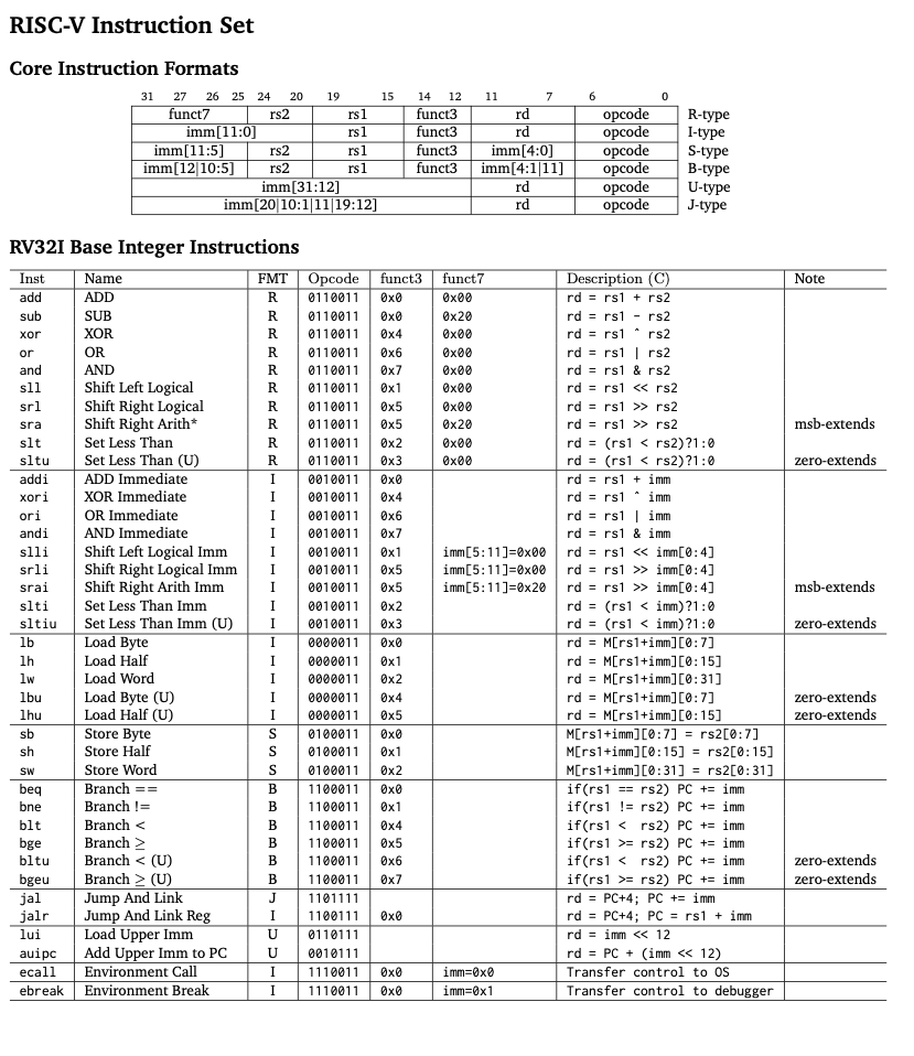
The codegenerator iterates over the generated IR and generates assembly code for each instruction. It traverses the IR tree and maps each node type to specific RISC-V instructions, and this isn’t a simple one-to-one mapping - it involves careful register allocation, stack management, and preserving calling conventions. Here’s how the process works:
IR Node → Register Allocation → Assembly Instructions → Function Prologue/Epilogue → Final Assembly
Call Node: For function calls, the code generator does the following:
Register Allocation: Incorporates a simple counter system (get_new_temp()) to allocate registers for temporary variables. It uses a stack-like approach to manage the registers, where the most recently allocated register is used first. For our “Hello, World!” program, the code generator would do the following:
Stack Management: Stack management is crucial for function calls. The code generator handles this by:
and the final compiled steps might look like this:
IR Node: Call: Some("printf")
     ↓
Assembly: la t0, .LC0    # Load string address
          mv a0, t0      # Set first argument
          call printf    # Call the function

IR Node: Return: None → Constant: Some("0")
     ↓
Assembly: li t1, 0       # Load immediate value 0
          mv a0, t1      # Move to return register
          # Epilogue follows
and the final assembly code would look like this:
.section .data
.section .text
.global main

.extern printf
.global main

main:
    # Prologue
    addi sp, sp, -8
    sw ra, 4(sp)
    sw s0, 0(sp)
    addi s0, sp, 8

.section .rodata
.LC0:
    .string "Hello, World!\n"
.section .text
    la t0, .LC0
    mv a0, t0
    call printf
    li t1, 0
    mv a0, t1
    mv sp, s0
    addi sp, sp, -8
    lw ra, 4(sp)
    lw s0, 0(sp)
    addi sp, sp, 8
    ret

    # Epilogue
    lw ra, 4(sp)
    lw s0, 0(sp)
    addi sp, sp, 8
    ret
The assembly code generated by Ferry is specific to the RISC-V architecture. It can be assembled into machine code using an external assembler like riscv64-unknown-elf-gcc and has to be linked with libc (C standard library) to create an executable binary. The assembly code is a low-level representation of the program that can be executed on a RISC-V CPU.
The process flows like this:
.s (Assembly code) --> Assembler --> .o (Object file) --> Linker --> Executable/ Machine code/ Binary
Ferry has a separate module that helps with the assembly and linking process. This is a separate binary that uses the
riscv64-unknown-elf-as to assemble and riscv64-unknown-elf-gcc tools to assemble and link the code. It then uses spike to run the code. The module is called mac_os_runner and the binary is called runner.
cargo run --release --bin runner -- <input_file.s>
The complete process of compiling and running a C program using Ferry in an ARM64 environment is as follows:
cargo run --release --bin ferry -- <input_file.c>
cargo run --release --bin runner -- <input_file.s>
Here’s a simple instruction decoder for RISC-V machine code
This tool helps you decode RISCV32I instructions and convert them to their corresponding assembly code. (for example, 00000000000000000000000010000011 to lb x1, 0(x0))
Here is the standalone version of the tool: Barney- A RISC-V Instruction Decoder. This is going to be a handy tool to understand the instructions and their working. The tool will also include decoding assembly code to machine code in the future. (an assembler for RISC-V instructions)
Yatch is a simple machine code interpreter for RISC-V. It can execute RISC-V assembly code directly, allowing you to run machine code directly on a simulated RISC-V CPU. Yatch was meant to show how CPUs read and execute instructions. Read everything about Yatch here.
Once you have the compiled assembly code, you can use a simulator like Yatch to simulate the execution of the code.
Well, the current scope of Ferry was to understand and demonstrate the working of compilers. While I would love to finish this, there are far better, superior compilers out there. This article was a simple entry into how systems work. My next steps would be delving more into the world of compilers, optimising CPU operations, and GPU computing, and understanding the mechanics behind the scenes.
Also, a big big shoutout to my boy, Claude 3.7 sonnet for improving the compiler and helping ship it 10x faster. Such a complex task would have taken me weeks, or even months, to complete. Claude wrote lines of redundant code - the extra parsing methods, a couple of functionality implementations in advanced optimisations and type checker functions that would have taken me a lot of time to finish manually. Especially the advanced optimiser. That part was a pain to write and Claude handled it like a pro. You still need a decent Rust knowledge to be able to fix whatever an AI model returns, but it did an excellent job.
This article might seem overwhelming, but it’s pretty interesting to realize how all of modern computing works and see how far we’ve come.